Optimal Weight and Learning Rates for Linear Networks
Regression Revisited
Suppose we are given a set of data (x(1),y(1)),(x(2),y(2))...(x(p),y(p)):
If we assume that g is linear, then finding the best line that fits the data (linear
regression) can be done algebraically:
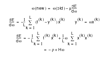
The solution is based on minimizing the squared error (Cost) between the network output and the data:
where y = w x.
Finding the best set of weights
1-input, 1 output, 1 weight
But the derivative of E is zero at the minimum so we can solve for
wopt.
n-inputs, m outputs: nm weights
The same analysis can be done in the multi-dimensional case except that
now everything becomes matrices:
where wopt is an mxn matrix, H is an nxn matrix and Á is an mxn
matrix.
Matrix inversion is an expensive operation. Also, if the input dimension,
n, is very large then H is huge and may not even b possible to compute. If we are not able to compute the inverse
Hessian or if we don't want to spend the time, then we can use gradient descent.
Gradient Descent: Picking the Best Learning Rate
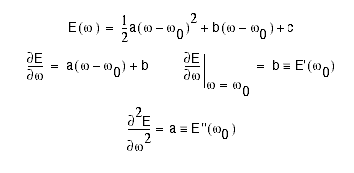
For linear networks, E is quadratic then we can write
But this is just a Taylor series expansion of E(w) about w0. Now, suppose
we want to determine the optimal weight, wopt. We can differentiate E(w) and evaluate the result at wopt, noting
that E`(wopt) is zero:
Solving for wopt we obtain:
comparing this to the update equation, we find that the learning "rate"
that takes us directly to the minimum is equal to the inverse Hessian, which is a matrix and not a scalar. Why
do we need a matrix?
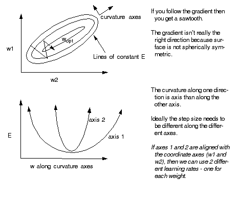
2-D Example
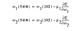
Curvature axes aligned with the coordinate axes:
m1 and m2
are inversely related to the size of the curvature along each axis. Using the above learning rate matrix has the
effect of scaling the gradient differently to make the surface "look" spherical.
If the axes are not aligned with coordinate axes, the we need a full
matrix of learning rates. This matrix is just the inverse Hessian. In general, H-1 is not diagonal.
We can obtain the curvature along each axis, however, by computing the eigenvalues of H. Anyone remember
what eigenvalues are??
Taking a Step Back
We have been spending a lot of time on some pretty tough math. Why?
Because training a network can take a long time if you just blindly apply the basic algorithms. There are techniques
that can improve the rate of convergence by orders of magnitude. However, understanding these techniques requires
a deep understanding of the underlying characteristics of the problem (i.e. the mathematics). Knowing what speed-up
techniques to apply, can make a difference between having a net that takes 100 iterations to train vs. 10000 iterations
to train (assuming it trains at all).
The previous slides are trying to make the following point for linear
networks (i.e. those networks whose cost function is a quadratic function of the weights):
- The shape of the cost surface has a significant effect on how
fast a net can learn. Ideally, we want a spherically symmetric surface.
- The correlation matrix is defined as the average over all inputs
of xxT
- The Hessian is the second derivative of E with respect to w.
For linear nets, the Hessian is the same as the correlation matrix.
- The Hessian, tells you about the shape of the cost surface:
- The eigenvalues of H are a measure of the steepness of the surface
along the curvature directions.
- a large eigenvalue => steep curvature => need small learning
rate
- the learning rate should be proportional to 1/eigenvalue
- if we are forced to use a single learning rate for all weights,
then we must use a learning rate that will not cause divergence along the steep directions (large eigenvalue directions).
Thus, we must choose a learning rate m that is on the order of 1/»max where »max
is the largest eigenvalue.
- If we can use a matrix of learning rates, this matrix is proportional
to H-1.
- For real problems (i.e. nonlinear), you don't know the eigenvalues
so you just have to guess. Of course, there are algorithms that will estimate »max ....We won't be considering
these here.
- An alternative solution to speeding up learning is to transform
the inputs (that is, x -> Px, for some transformation matrix P) so that the resulting correlation matrix, (Px)(Px)T,
is equal to the identity.
- The above suggestions are only really true for linear networks.
However, the cost surface of nonlinear networks can be modeled as a quadratic in the vicinity of the current weight.
We can then apply the similar techniques as above, however, they will only be approximations.
[Top]  [Next: Summary]
  [Back to the first page]


![]()
![]()


